Table of Contents
Introduction
Viasat Inc. is an American communications company that provides high-speed satellite broadband services and secure networking systems covering military and commercial markets. Therefore, ensuring high quality network performance is crucial for maintaining customer satisfaction. Fundamental factors that affect network performance are packet loss and latency.
Small units of data that are sent and recieved across a network are called packets, and packet loss occurs when one or more of these packets fails to reach its intended destination. Latency is the delay between a user's action and a web application's response to that action. High quantities of each of these often results in slow service and network disruptions for the user.
The problem we are trying to explore is: can we detect anomalies within network traffic, whether it be an increase in the packet loss rate, larger latency, or both? Packet loss can be caused by a number of issues, including: network congestion, problems with network hardware, software bugs and security threats. On the other hand, main factors that affect network latency are: the transmission medium (copper cable-based networks vs. modern optic fibers), propagation (how far apart the networks are), efficiency of routers and storage delays.
The ability to detect anomalies on a data stream would be extremely useful as it can be an effective monitoring & alerting system for poor network conditions. If an anomaly is predicted, our hope is that a proper recovery protocol can be put in place to stabilize network performance, creating a better experience for the end user.
Methodology
The Data
We will be using data generated from DANE (Data Automation and Network Emulation Tool), a tool that automatically collects network traffic datasets in a parallelized manner without background noise, and emulates a diverse range of network conditions representative of the real world. Using DANE, we are able to configure parameters such as latency and the packet loss ratio ourselves. More importantly, we are able to simulate an anomaly by changing the configuration settings of the packet loss rate and latency mid run. The data collected is already aggregated per second with these fields:
| DANE Features | Description |
|---|---|
| Time | Broken down into seconds(epoch) |
| Port 1 & 2 | Identifier of where the packets are being sent to and from. Can originate from either |
| IP | IP address of the ports in comunication |
| Proto | IP Protocol number that identifies the transport protocol for the packet |
| Port 1->2 Bytes | Total bytes sent from port 1 to 2 in given second |
| Port 2->1 Bytes | Total bytes sent from port 2 to 1 in given second |
| Port 1->2 Packets | Total packets sent from port 1 to 2 in given second |
| Port 2->1 Packets | Total packets sent from port 2 to 1 in given second |
| Packet_times | Time in milliseconds that the packet arrived |
| Packet_size | Size of the bytes of the packet |
| Packet_dirs | Which endpoint was the source of each packet that arrived |
We ran only two scenarios at once to prevent overloading our CPU by running too many DANE scenarios concurrently. Each DANE run is 5 minutes long. The configuration change happens at the 180 second mark and what we configure for our packet loss rate determines the likelihood of each packet being dropped. This way, we are able to simulate an anomaly within our data and are able to simulate packet loss in a more realistic manner. Our steady state had a packet loss ratio of 1/5,000 and a latency of 40 ms. We are focused on identifying changes of a factor of 4 and above. In our case a packet loss ratio of 1/1,250 and a latency of 160 ms or greater or a packet loss ratio of 1/20,000 and latency of 10 ms.
Definition of an Anomaly
The type of behavior we are looking for is different from what a conventional anomaly would behave like. Typical anomalies are characterized by significantly large spikes or drops in a feature. The behavior we are looking for is more closely related to anomalous regions where the degradation in the network continues; these anomalies resemble shifts. As we will show in the next section, spikes in our features that would normally resemble anomalous behavior are perfectly random and not caused by any change in network quality. These anomalies would be considered false positives if detected.
EDA and Feature Engineering

Figure 1 The packets per second sent from machine 1 → 2 with conditions of 50 ms latency and 1/2500 packets expected to be dropped with the conditions shifting to 300 ms latency and 1/1250 expected packet drops at 180 seconds.
Comparing last quarter’s deterministic packet drops data with this quarter’s random packet drops data, we can see that the correlation between packets per second and packet loss is still there. Since packet loss and latency are our only ways of generating an anomaly, features such as packets per second and other features correlated with packet loss and latency will be our basis for determining whether there is an anomaly or not.
Exploring Packets Per Second Feature
| First 180 Seconds | Last 120 Seconds | |
|---|---|---|
| Mean | 1783.72 | 428.43 |
| Standard Deviation | 710.10 | 260.22 |
| Max | 4404 | 1548 |
| Min | 680 | 152 |
Exploration of Anomaly Detection Methods
I. Forecasting
Since we are dealing with time series data, we can create an anomaly detection model through the use of forecasting techniques. The basic concept is that we will pick a feature, in this case total packets sent per second (volume of traffic) and build a forecast. If the expected value is outside of our prediction interval (threshold) we will flag it as an anomaly. We are employing a multivariate time series forecast because we are using predictors other than the series (a.k.a exogenous variables).
We will be focusing on building an ARIMA (Auto Regressive Integrated Moving Average) model. This model is actually a class of models that ‘explains’ a given time series based on its own past values, that is, its own lags and the lagged forecast errors, so that equation can be used to forecast future values.
An ARIMA model can be characterized by 3 terms:
- P: Order of the “AR” term which refers to the number of lags of Y to be used as predictors
- A pure Auto Regressive (AR only) model is one where Yt depends only on its own lags. That is, Yt is a function of the ‘lags of Yt’.
- A pure Auto Regressive (AR only) model is one where Yt depends only on its own lags. That is, Yt is a function of the ‘lags of Yt’.
- Q: Order of the “MA” term which refers to the number of lagged forecast errors that should go into the model
- Likewise a pure Moving Average (MA only) model is one where Yt depends only on the lagged forecast errors.

- Likewise a pure Moving Average (MA only) model is one where Yt depends only on the lagged forecast errors.
- D: Number of differencing required to make the time series stationary
An ARIMA model is one where the time series was differenced at least once to make it stationary and you combine the AR and the MA terms. So the equation becomes:

To hypertune these parameters of (p,d,q), we performed a grid search method and chose our model based on the AIC (Akaike Information Criteria). The AIC is a widely used measure of a statistical model. It basically quantifies 1) the goodness of fit, and 2) the simplicity/parsimony, of the model into a single statistic. When comparing two models, the one with the lower AIC is generally a “better-fit model”.
To simulate a live stream of data, we chose to implement window intervals of n seconds to train our ARIMA model on. We found that window intervals of 20 seconds worked best. Therefore, we aggregated our data into 20 second intervals with the mean of the total packet sent as our feature. Our training data consisted of eighteen 5 minute DANE runs for a total of approximately an hour and a half of network traffic. The first 30 minutes of data is our steady state with a latency of 40 ms and a packet loss ratio of 1/5000. Afterwards, we had 5 separate, spaced out instances of simulated anomalies with a return to a steady state in between each case. Each anomaly in our training data changed the latency to 160 ms and the packet loss ratio to 1/1250.
To flag anomalous behavior, we calculated a 99% prediction interval around each forecast. If the actual value falls outside this interval, it is flagged as an anomaly. We tuned our prediction interval range from 95% - 99% and found that a 99% prediction interval was a wide enough range to limit the amount of false positives and capture extreme anomalous behavior. In addition, we also log transformed our data (mean of the total packets sent) to reduce the scale because the original data range was in the thousands and since our model considers forecast errors as part of the model, our prediction interval was much too wide. By transforming the data onto a smaller scale, we are better able to capture anomalies.
 Figure 2 ARIMA model anomaly detections using a 99% CI on the training set. The conditions generating the data: 40ms latency and 1/5000 packets dropped shifting to 320ms latency and 1/1250 packets being dropped. Time is measured in units of 20s since the ARIMA model trains on 20s aggregations of packets per second as a single data point.
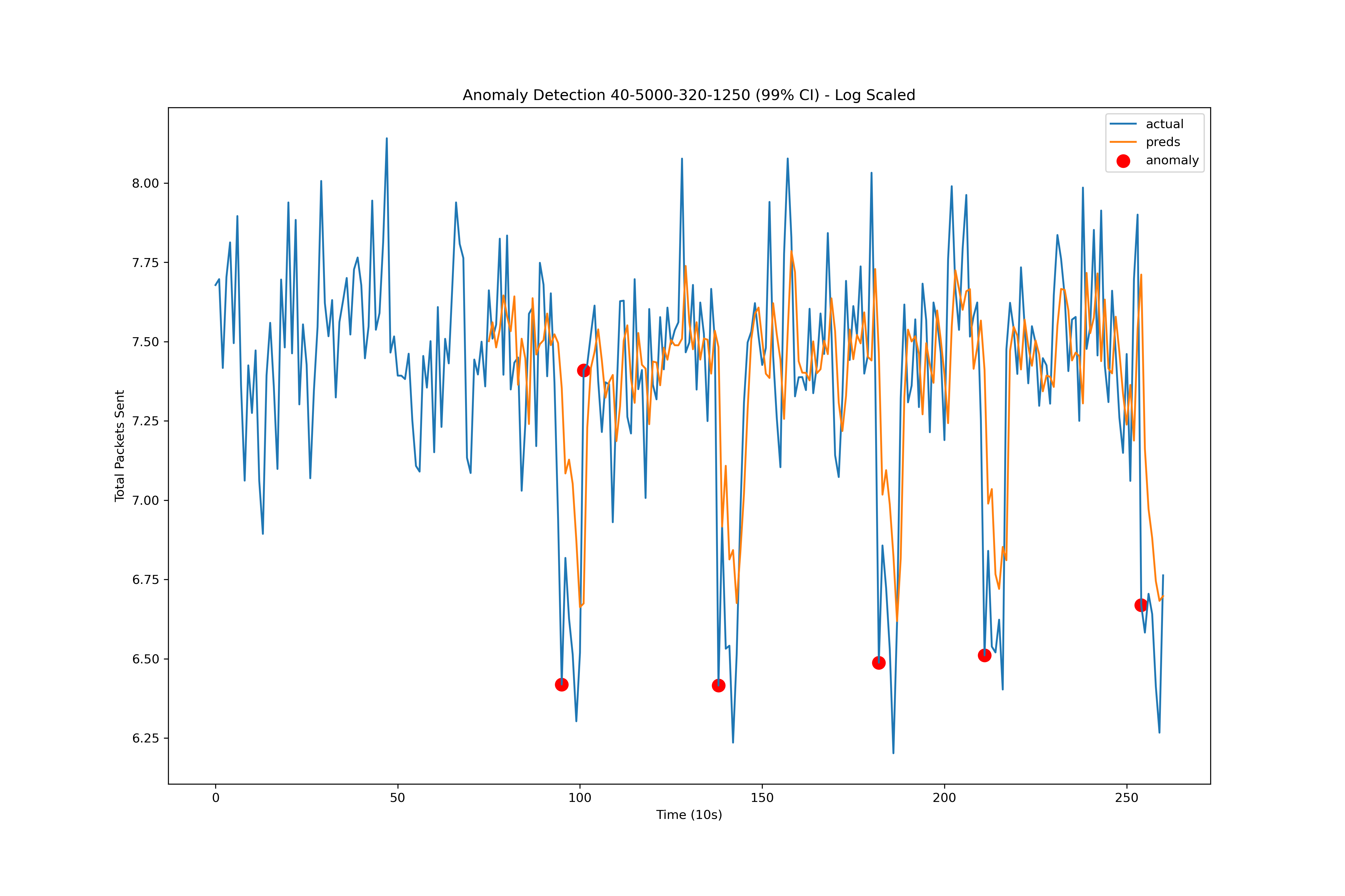 Figure 3 ARIMA model 99% CI predictions on training data with a log scale. The conditions generating the data: 40ms latency and 1/5000 packets dropped shifting to 320ms latency and 1/1250 packets being dropped. The ARIMA forecasts can be seen in orange.
We then ran the model on our test set concatenated to our train data. We can see in figure 4 that there were 2 instances of false negatives where our model did not flag the configuration change as an anomaly. There was also a large spike in the middle of our steady state traffic which was flagged as anomalous, representing one case of a false positive. This window of traffic just so happened to have an extremely large volume of packets sent and was not due to a configuration change.
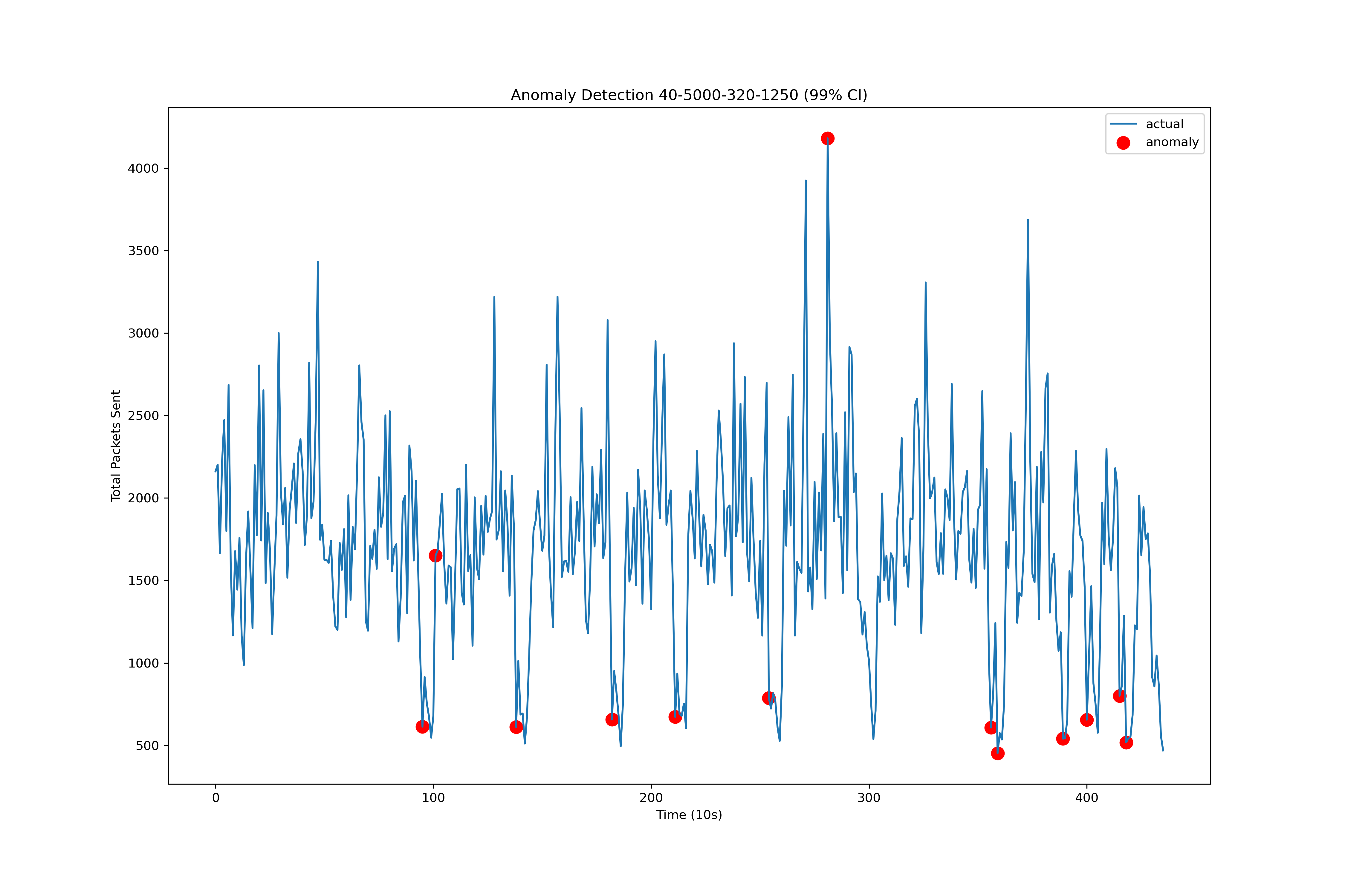 Figure 4 ARIMA model anomaly detections using a 99% CI on the test set. The conditions generating the data: 40ms latency and 1/5000 packets dropped shifting to 320ms latency and 1/1250 packets being dropped. Time is measured in units of 20s since the ARIMA model trains on 20s aggregations of packets per second as a single data point.
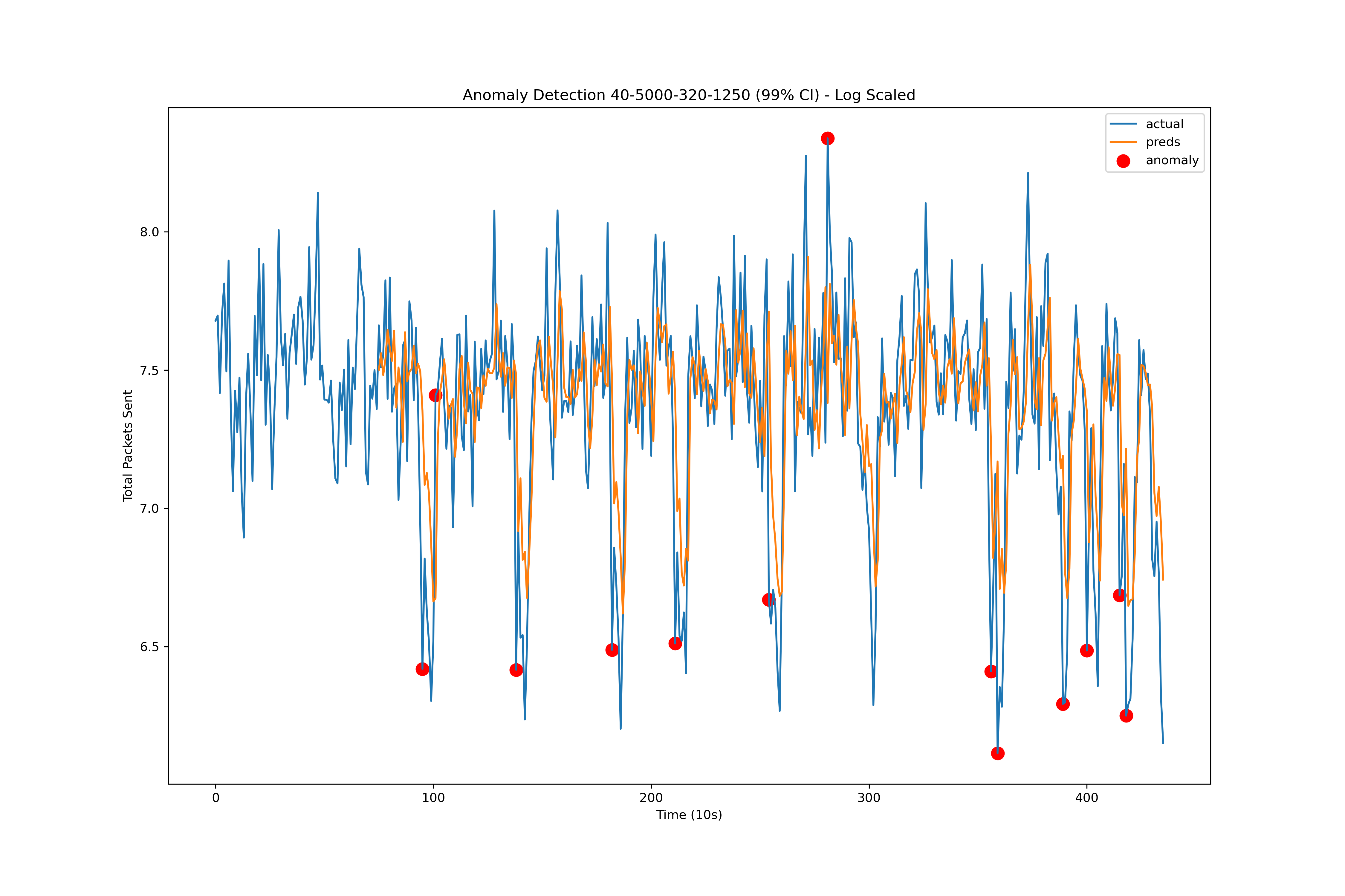 Figure 5 ARIMA model anomaly detections using a 99% CI on the test set with a log scale and forecast predictions.
II. MAD & Median
The Median Absolute Deviation based model tries to take advantage of the differences in the features of spikes and shifts in a time series. Median and median absolute deviation are transformations to the 1 → 2 packets per second data using a rolling window. Some properties of this transformation: smoothens out the data, depending on the window size median and MAD is robust against spikes, is sensitive to shifts in the data. Median and MAD depend on the assumption that spikes are relatively short and uncommon, and shifts are persistent. When a spike occurs the median would remain almost unchanged since the data points outside the spike would make up more than 50% of the window same applies to deviation from the median, hence why larger window sizes tend to do better. Shifts in the data on the other hand eventually result in a shift in the median since they persist much longer than 50% of the rolling window size.
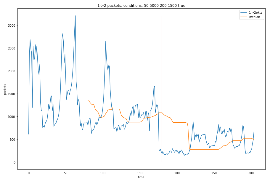 Figure 6 Median applied on a rolling window with a window size of 80 seconds. The median at a given time is the median of the previous 80 seconds of data. The red line represents the time the shift in packet loss and latency happens.
The model determines if a data point is an anomaly if a transformation of the median and MAD are above a threshold based on the window size. The threshold is determined by 100/window size. Deviation from the median was included in the transformation to limit the effect of large variance in the window. If there is a lot of variance but no shift, the data would be above and below the median so the sum of the deviations would be low in magnitude but in a shift the data would be either strictly above or below the median and result in a high magnitude. All of these transformations that picked at differences between spikes, shifts and data with high variance in a window would be combined to make the presence of a shift more apparent. The transformation used was:
![]()
Where MAD is median absolute deviation and DM is the sum of the deviation from the median
The MAD model takes in the 1 --> 2 packets per second data output by DANE and applies the transformation above on a given window size. As we can see with the transformation the spikes in the beginning of the run get flattened out while the shift beomes a spike in the transformation and easy to detect.
![]() Figure 7 Transformation of the 80 second rolling window on the data in figure 6. The purple line is the threshold used to determine an anomaly, it is 100/window size. The anomaly gets detected at ~220 seconds.
Figure 7 Transformation of the 80 second rolling window on the data in figure 6. The purple line is the threshold used to determine an anomaly, it is 100/window size. The anomaly gets detected at ~220 seconds.
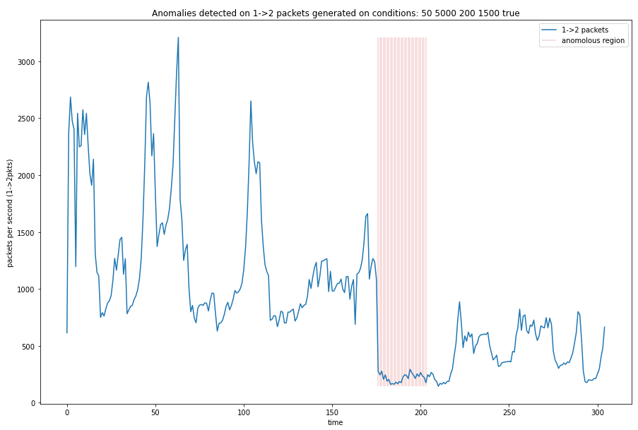 Figure 8 Shifting the time the anomaly was detected on the transformation by half of the window size (40 seconds) we can observe the spike in the transformation corresponds to the shift in the 1 –> 2 packets per second data.
Since the model uses a rolling window to determine the anomaly the detection is delayed by a function of the window size. Shifting the detection by half the window size lines up the alerts with the shift.
Results
Performance Measures
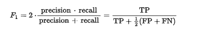
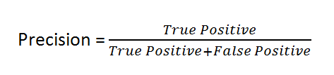
We chose to use F1 score as our metric but also considered precision in our metrics. Our motivation behind choosing F1 score and precision is because anomalous regions cause by network degradation are assumed to be rare. Since the intended use for this ensemble model is to alert ISP employees what connections are degraded if too many false positives are being flagged then there would not be much use in the alarm.
Our goal is to have the users trust that if there is an alarm they can be sure that there is network degradation, hence why precision is considered. We also do not want our model to always predict negative, making it trivial so F1 score was included.
| F1 Score Formula | Precision Formula |
|---|---|
 |
 |
Performance
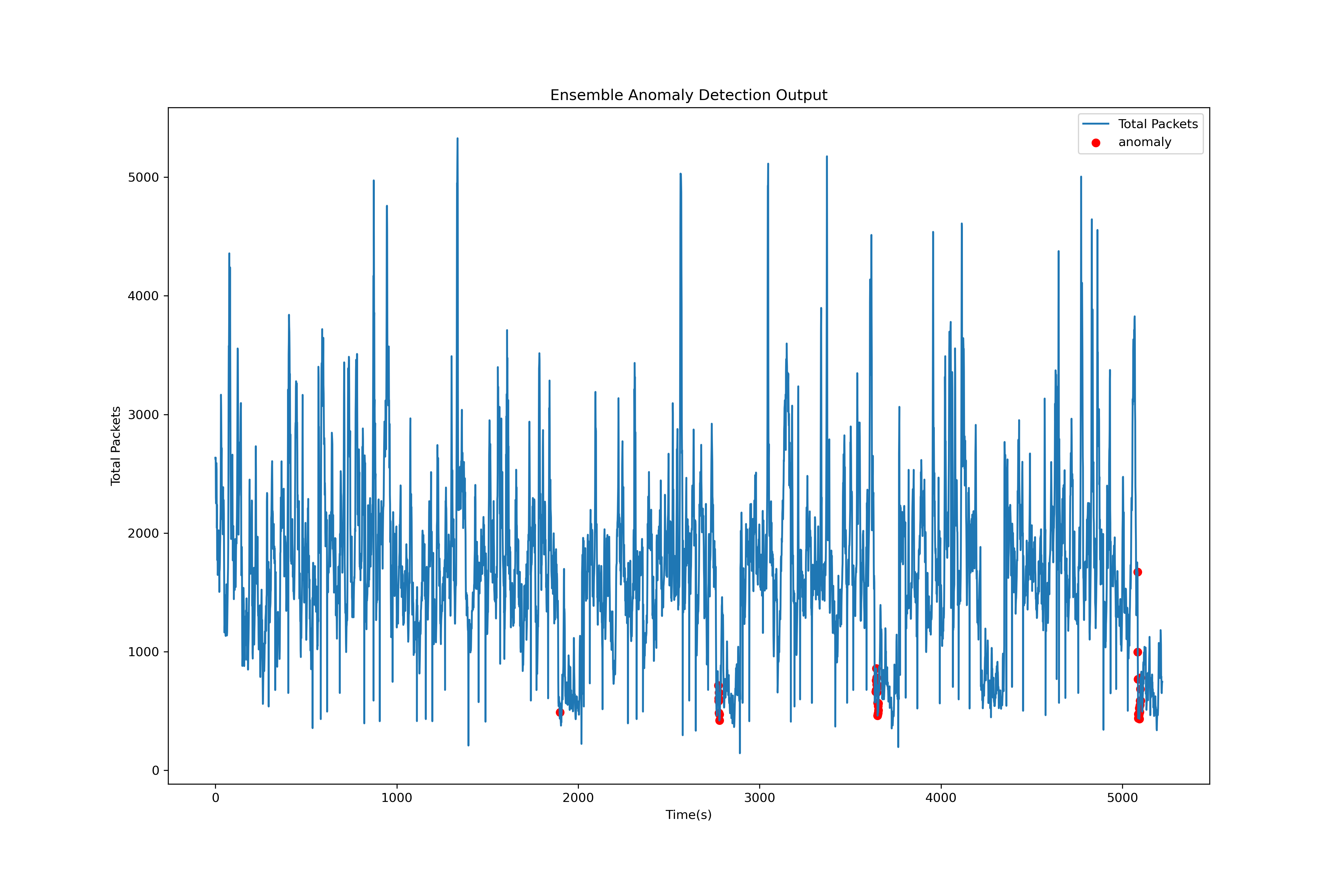
Our method to combine our ARIMA and MAD model followed a simple logic. We ran both models independently and compared the results of each model. We used an AND operator to see where both models detected an anomaly and labeled it as an anomaly. Otherwise, if the condition is not met, then we do not label it as an anomaly.
Using the ensemble logic described above, our results show that we are able to detect anomalies early on when they occur. However, we have one false negative where no anomaly appears due to the fact that our ARIMA model detects the anomalies early on but the MAD model detects the anomalies later, so there is no overlap for our ensemble logic to agree on an anomaly.
Future Work
Bigger Questions
One of the assumptions made about anomalies was that they strictly decrease network quality so the packet loss ratio always increased and the latency always increased. When creating training and testing data several separate DANE runs were stitched together to see the performance with several drops in network quality but a recovery process was never run. The runs went from the end of one run at low network quality to the begining of another DANE run at normal network quality. This "recovery" process from stitching DANE runs together may not be representitive of real network behavior and false positives may result from the difference in behavior.
Improvements
A major portion of work that our group was not able to venture into was to generate a more realistic dataset to test our model on. Our methodology of concatenating multiple runs of DANE to “simulate” about an hour and a half of network traffic is not exactly accurate because we do not know if networks jump back to a steady state as quickly and abruptly as shown in our dataset. Also, we were only able to train and test our model on one configuration for our steady state which was a network with a latency of 40 ms and a packet loss ratio of 1/5000. It would have definitely been interesting to see how our model would perform on a test set with a new steady state so we can further hypertune our model. For example, the ARIMA model only uses “total packets” as its feature and we know from our results from last quarter that different latency and packet loss ratios results in different behavior for total packets sent over the network. Therefore, the parameters for our ARIMA model would most likely change if our steady state changes.
As we have it right now, our ARIMA model is only trained on one configuration so an addition we would have to make is to continuously or periodically retrain the ARIMA model to make sure that it is correctly hypertuned. Moreover, our ensemble logic was very naive and rough and it would’ve been extremely useful to flush our ensemble model out even further. As we currently have it, our MAD model is hypertuned to have a window size of 80 seconds while our ARIMA model is hypertuned to take in inputs of 20 seconds. The different inputs of each model may need the development of different data pre-processors for each.
References
- https://towardsdatascience.com/outlier-detection-with-isolation-forest-3d190448d45e
- https://towardsdatascience.com/anomaly-detection-with-isolation-forest-visualization-23cd75c281e2
- https://www.machinelearningplus.com/time-series/arima-model-time-series-forecasting-python/
- https://people.duke.edu/~rnau/411arim.htm
- https://coolstatsblog.com/2013/08/14/using-aic-to-test-arima-models-2/